LA188 Final Project:
Irrigation and the High Plains Aquifer
I. Forming some questions
It's easy to obtain large volumes of data,
especially from federal agencies, but not so easy to understand it well enough
to ask meaningful questions. Therefore I turned to my advisor, Professor
Patzek, for help. He suggested investigating the sustainability of
grain production in the US, in particular the dependence on irrigation from the
High Plains aquifer, which is substantially depleted in parts. Some questions
that could be asked:
- How is the intensity of agriculture correlated with the rate of withdrawal
of water? Can we measure the value of the resource that is being extracted?
- Which areas are most at risk for increased cost of food production as the
water level drops?
Background
The High Plains aquifer makes possible today's large-scale agriculture in
regions that were too dry to farm before mechanized pumping. It lies under parts
of eight states, and stores a volume of water about as large as one of the Great
Lakes. This
"fossil water", the remains of melted glaciers from the last ice age, had been stored for thousands of
years until the development of irrigation starting in the 1940's. Because of its
economic importance, the aquifer is intensely studied by the USGS; this
background comes from their reports:
II. Outline of solution
- Find data on water use, aquifer levels, and farming at as fine a
resolution as possible, which turns out to be the county level.
- Calculate average drawdown of the aquifer in each county.
- Graph the market value of crops versus the rate of withdrawal from the
aquifer and the amount of drawdown.
- Identify the least sustainable regions, where there is both intense agriculture and rapid fall of the water
table.
III. Finding data
An excellent place to start is the National
Atlas download site, which organizes geographic data from many federal agencies.
- Agriculture: The summaries at the National Atlas
turned out to be not detailed enough, so I followed their link to the
source, Census
of Agriculture, which publishes statistics derived from surveys
mailed to all known farms in the nation. The census is taken every five
years, most recently in 2002 and 1997. (Selected statistics are shown on national
maps.)
The statistics are reported by
county, but sometimes data is withheld when there is only one farm reporting
in a county, because of confidentiality. A shapefile of county boundaries is
available, but I decided not to use it because (according to its metadata) it is intended for display at
a national scale, 1:20,000,000 or smaller, so the county boundaries were too
simplified and crude for the scale I wanted to work at. For example, here's
what Maryland looks like zoomed in to 1:3,000,000:
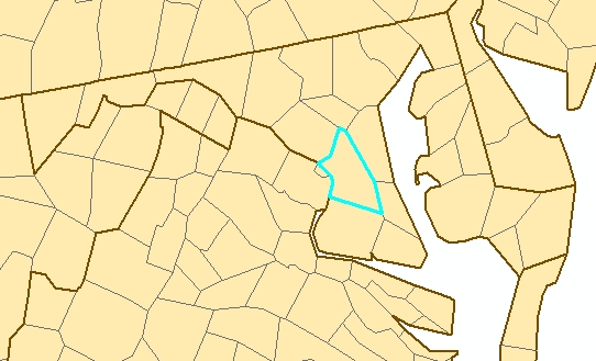
Notice that Washington, DC does not exist on the map; it has been subsumed
into the neighboring county (highlighted). Therefore, I downloaded only the Data
Query Application, which was a very convenient way to extract attribute
tables with only the attributes I wanted; these table will be joined to a
more detailed shapefile. The statistics I'm most interested in are
- corn production in bushels
- number of irrigated acres of corn
- market value of crops, and of grains as a subset of crops
- High Plains Aquifer: The first Google hit on "High Plains Aquifer" is
the High Plains Aquifer Information
Network, an academic site which links to the USGS High
Plains Regional Ground Water Study, where many GIS
data sets are posted, and also to the lookup
of USGS datasets by theme "High Plains Aquifer". I
got these datasets:
| Contents |
Filename |
USGS location |
Format |
Coordinate system |
Comment |
| Aquifer boundary |
aqbound |
ofr99-267 |
coverage |
GCS_North_American_1983 |
|
| County boundaries at 1:100,000
scale, clipped to the High Plains region. |
hpcountys |
hpcountys |
shapefile |
NAD_1927_Albers |
Metadata is in
HTML, can't import it! |
| State boundaries
at 1:100,000, clipped to the High Plains region. |
hpstate |
hpstate |
shapefile |
NAD_1927_Albers |
|
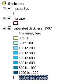
| Saturated
thickness of aquifer, 1996-97 |
sattk_97 |
ofr00-300_sattk9697 |
shapefile |
NAD_1927_Albers |
|
| Water level changes 1980-1997 |
wlc80_97 |
ofr00-96_wlc80_97 |
coverage |
NAD_1927_Albers |
|
See footnotes on downloading.
- Water Use: I looked on the National Atlas under Water, and they
provide tables of water use gathered by the USGS
Water Use Information Program, showing water use by county in categories
including public supply, irrigation, industrial, etc. The source of data on
irrigation is chiefly State and Federal crop reporting programs, as well as
estimates based on irrigated acreages and application rates (see
discussion). This is very useful,
since the Agriculture Census reported only the number of irrigated acres,
not the actual amount of water used
for irrigation. I
downloaded the water use tables for 1995 and 2000, with their metadata.
- Rivers: I got the linear hydrography features from the National
Atlas and clipped it to the county boundaries layer. There are too many
water features to show on the map at the regional scale, so I selected the four most
important rivers (as shown on maps in the USGS
report) and exported them as a layer.
IV. Putting all layers in the same datum and projection
The USGS shapefiles did not come with .prj files, but the projection
was given in the metadata, so I could define it by hand. The coverages do have projection defined
in a way that ArcMap recognizes. Most of the USGS layers used an Albers Conical Equal Area
projection with NAD1927 datum, USGS version:
| standard parallel |
29.5 |
| standard parallel |
45.5 |
| longitude of central meridian |
-96 |
| latitude of projection origin |
23 |
| false easting |
0 |
| false northing |
0 |
I transformed the only one that was different to
this coordinate system. The rivers layer was in geographic coordinates with
NAD1927 datum; ArcMap automatically projects it to the data frame's projection.
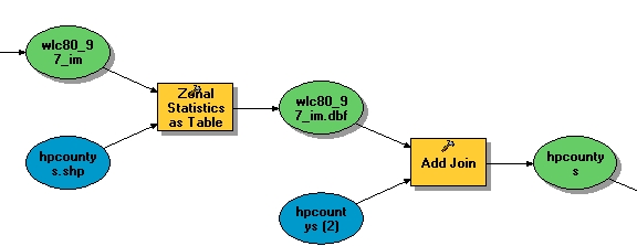
V. Data Processing
ArcMap's Model Builder was helpful for keeping a record of exactly what steps
I went through and which options were used in each tool.
-
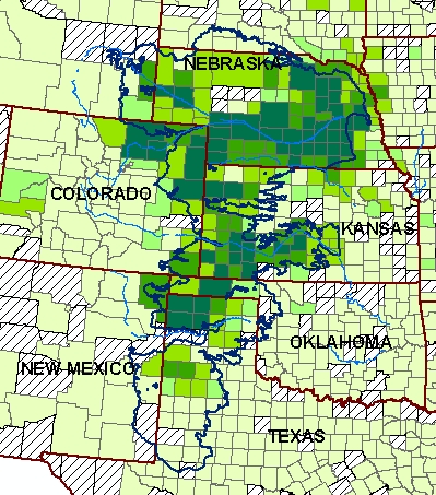
Join the county layer to the agriculture tables. (Footnote on
joining tables) The map
below shows the number of
irrigated acres of corn in 2002. The irrigated acreage follows the shape of the aquifer
quite closely, and also clusters around the major rivers, Platte
River in Nebraska and Arkansas River in Kansas.
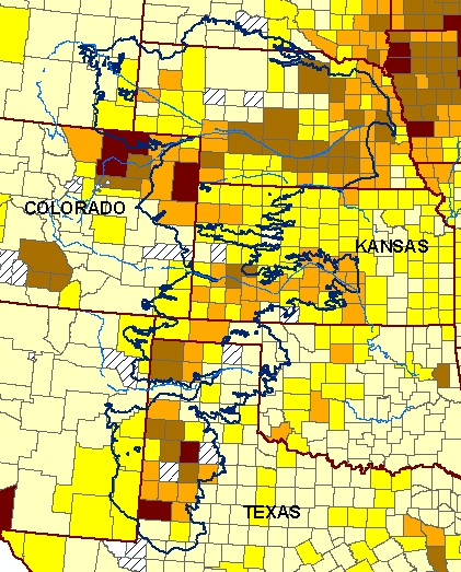
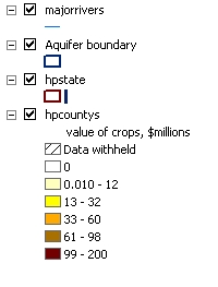
And this map shows the market value of all crops in 2002. It looks like
in Nebraska corn dominates the crops, while in Texas there is
some other crop being grown besides corn to get high market values
(from looking into the data tables, that other crop is cotton). The value of crops is clearly higher inside the aquifer
than outside in Kansas, Colorado and Texas. To the northeast in
Iowa, there is more rainfall and high market values are achieved
with much less irrigation.
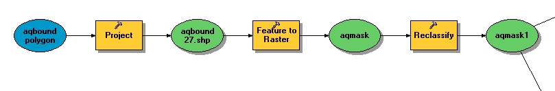
- The aquifer boundary will be needed as an analysis mask for
working with rasters. First, it needs a datum transformation to use
the same datum, NAD27, as the other layers. The Project tool takes
only the polygons, not the entire coverage, and writes a new
shapefile. Next, convert it to a raster; I chose a cell size of 1000
meters because it is a convenient round number that is a little
smaller than the resolution of the feature layer, judging by zooming
in and looking at it. The raster value is taken from the OUTCROP
attribute, which is 0 for the main aquifer polygon and 1 for other
polygons representing small holes within it where the aquifer is not
present. Finally, the 1 values are reclassified to NoData so it can
be used as a mask.
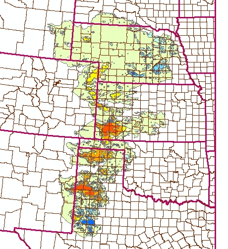
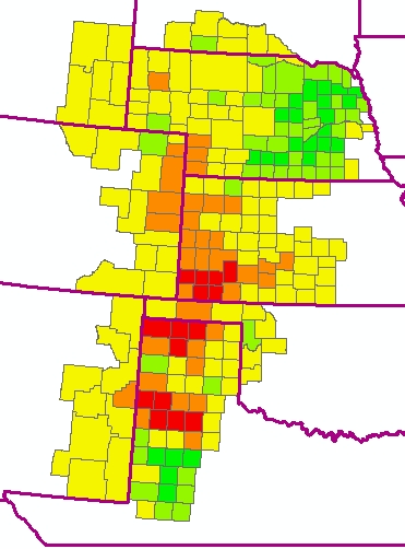
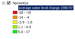
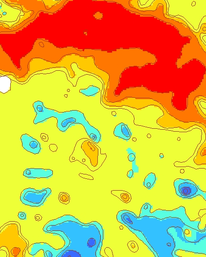
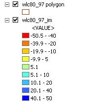
- The water-level layer contains contours of water-level changes
from 1980 to 1997 in feet. According to the USGS
report, the irrigated acreage and the rate of withdrawal
remained roughly the same during that time, after a large expansion
of irrigation from 1940-1980. Note the large declines in the water
level in southwestern Kansas and the Texas panhandle, while in
eastern Nebraska the water level has increased, due to wetter
conditions.
This change should be compared to the saturated thickness remaining
in the aquifer as of 1997:
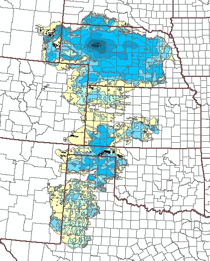
It appears that in Texas there are only a few decades worth of water
remaining, based on drawdowns of 40 feet in two decades and
remaining thickness of around 100 feet. Only about 60 to 80 percent
of the water can be fully extracted with pumps, because some of it
remains bound in the pore space due to capillarity, and a large
capacity well requires a minimum of about 30 feet of saturated
thickness to operate; see the USGS
report.
-
I want to get the average values over each county. First I
need to interpolate to a surface. Topo To Raster seems to be the
appropriate tool: it is intended to interpolate from contour lines
with a spline-based method. Other options would be extracting the vertices to make a points layer, then
interpolating with a method such as spline or inverse distance
weighted, or making a TIN, but
these would require more steps.
- These contours were originally created as follows: (from
metadata) "Water-level points for 5,233 wells were reviewed and then
printed on mylar with the aquifer boundary ... Contours were then handdrawn using
an interpolated grid from ARC/INFO... The interpolation method used in ARC/INFO was Kriging with
the universal1 method." For a more in-depth project, it
would be better to contact the USGS to obtain the original point
feature layer for the wells and interpolate a surface from that.
- Some contours have a code "99"
which isn't a real data value, but probably means the
contour encloses
an "island" where the aquifer is not present. There are
only 3 of these and they are small, so I decided to ignore them
by selecting only contours with MAJOR1_POLY < 99 and making a
feature layer.
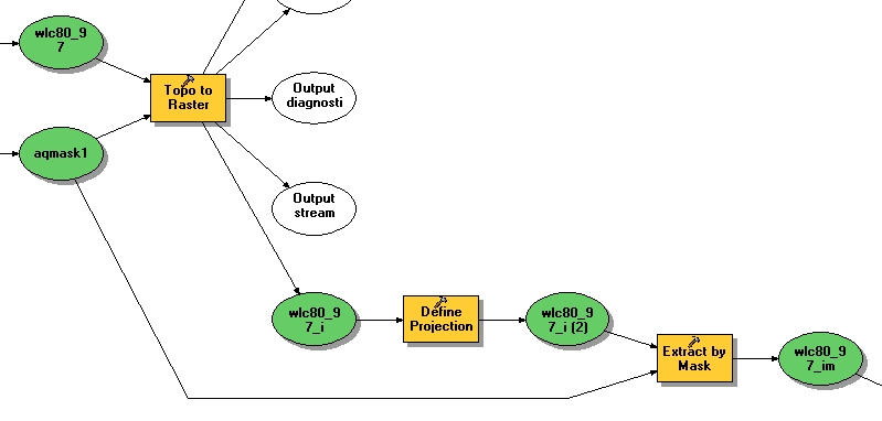
- Interpolate with Topo to Raster, with the drainage
enforcement option turned off, because it is meant for terrain
elevation. See the ArcMap help screens for explanation. Strangely, ArcMap didn't record the coordinate system for the
interpolated layer, so again I have to define projection and
import the coordinate system from the original feature layer. It should have done that automatically.
- Use Extract by Mask to mask out all cells where the aquifer
is not present.
Here's how the interpolated and masked surface appears.

- Use Zonal Statistics to find the average drawdown
over each county. (Use the Ignore NoData option to take the average
only over the cells in the county that belong to the aquifer.) Join
the statistics table to the county table, and uncheck Keep All to
keep only the counties that appear in the statistics table, that is,
the 235
counties that overlap the aquifer.
This produces a map of average drawdown in each county:
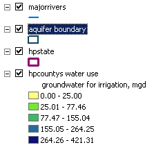
- Join water-use data for 2000 to the county layer. This map shows withdrawal of groundwater for irrigation, in millions
of gallons per day, by county. Notice that the greatest withdrawal
rates are not necessarily in the same places as the greatest
water-level drops. A full description of the flow of groundwater in
the aquifer would require software beyond ArcMap, such as Modflow,
another USGS product.
- Finally, join all the tables, select the 225 counties that both
overlap the aquifer and have valid data for value of crops,
and export a combined layer for making graphs.
V. Conclusions
Using the joined table, the variables of interest can be plotted against each
other.
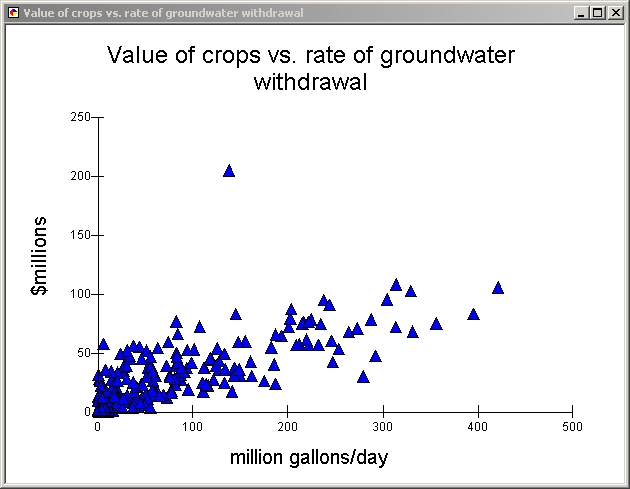
Clearly there is a very strong correlation between groundwater withdrawal and
market value of crops in the aquifer, except for the one outlier (Weld County,
Colorado, which barely overlaps the aquifer).
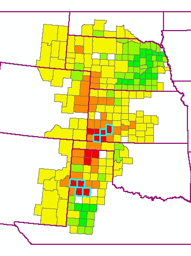
In the next map, counties are selected that have high intensity of
agriculture (> $50 million market value of crops, a round number that is about the
highest 25% of counties) and large water level drop (below -15 feet, about the
lowest 25%). These could be considered counties at the greatest risk of
spiraling costs of irrigation as water must be raised from greater depths.
The real issues are how much depth remains in the aquifer at these locations, how much
longer it will last at current withdrawal rates, how the cost of pumping
will increase with time and oil prices, and how
successful farmers have been at increasing efficiency of irrigation. Check out
the USGS report for deeper consideration of these
questions.
VI. Data Quality and Uncertainty
The major limitation of this analysis is that most data was only available at
the county level, and a county is a very large area (compared to a farm) and its
boundaries are irregular and not necessarily related to any natural features of
the data. I'm not sure how to quantify the resulting error; I would need some
information on the variation of land use within a county. Many counties barely
overlapped the edge of the aquifer, although there might be another different
aquifer within their boundaries. It might have been more valid to exclude
counties that are not wholly within the aquifer.
Other data quality issues:
- Missing data in the water use and agriculture tables. In the agricultural
census, some data was withheld for confidentiality. Also, the census was
based on a mailed survey, which can't achieve 100% completeness, although
they have detailed procedures including followup on missing data for farms
known to be large or unique. See the census
report for discussion of survey completeness, sampling strategy, and
calibration for missing data.
- The water use and agriculture data are from different years, 2000 vs.
2002, and 2000 was noted to be an especially dry year.
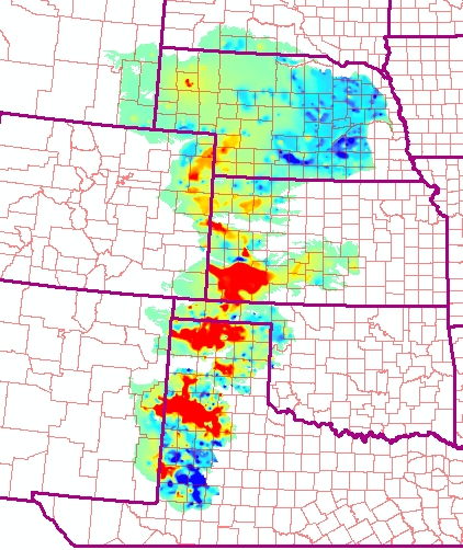
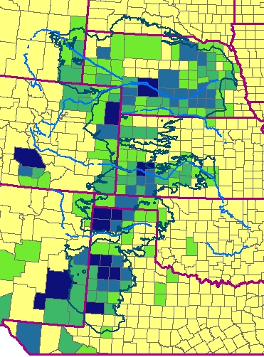
- The interpolation of a surface from the contours of water-level change
results in uncertainty. Different interpolation methods would give varying
results. One way to check the result is to compare the interpolated surface
with the original contours:
Some of the small bumps and holes were smoothed out by the interpolation.
However, the effect of such errors on the average over an entire county is
probably less important than the uncertainties discussed above. To improve
the accuracy of the water-level surface, it would be better to obtain the
original point data from the sampling wells, rather than tweak the
algorithms for interpolating from contours.
Footnotes
- Notes on downloading:
- For coverages, unpack the
.e00 file (ArcInfo interchange
format) with ArcCatalog as described in Lab
6.
- Shapefiles are compressed and require the
tar
utility to extract them. Fortunately it is installed in the Wurster Hall
PCs under the Hummingbird Connectivity package. Caution: unix tar
extracted only part of the files, and produced damaged files that could
not be transferred by SSH Secure Shell, nor opened by ArcMap.
- Import metadata, using ArcCatalog Metadata toolbar. Metadata is
usually found on the same website with the data in
.xml or .txt
form.
- ArcCatalog also handles metadata for data tables. The water use
tables came with their metadata, which
explained the cryptic field names and gave units. It required some hand editing: for example, ArcCatalog didn't recognize that
"Ps-wgwfr" in the metadata should refer to field name
PS_WGWFR.
- The agriculture query tool produces text files which explain the
column headings and attribute values (units of numbers, codes in
flag columns), but they are not in a standard format that ArcCatalog
can import. I hand-edited some of the field names using Excel, but
mostly didn't bother.
- Joining the tables took some fixing.
- The join attribute is the five-digit code that
identifies US counties, defined by the Federal Information
Processing Standard (FIPS). The shapefile has this code as an
integer, while the other tables have it as a string. I had to add a new
integer field to the water use table, and calculate its value from the string
FIPS. Fortunately, this works.
- Each agricultural data column has a corresponding flag column
indicating whether a zero value of data is a true zero or represents data withheld for confidentiality. In order to symbolize
the data on the map, I needed to put a code for withheld data in the data column. I selected the
withheld rows by attribute, clicked Show Selected, then used
Calculate Values in
the data column to set them to -1.
- To make it easier to work with joined tables, select only the
desired fields in the Fields tab of the Layer Properties, then
export the data as a new table, which will have all the desired
joined fields and none of the extraneous ones. However, I couldn't
find out how to do this in ArcToolbox, so I couldn't record this
step in Model Builder.
- Join all the tables first and then join the result to the
shapefile, to avoid making unnecessary copies of the spatial data.