Separating Different Sources of Data: Spacing Algorithm Succeeds where Standard Deviation Threshold Fails

Suppose you have a sample of data which may not all be drawn from the same distribution. Most of it, here called "regular data", comes from some continuous distribution with a decaying right tail, with no fixed maximum possible value. But there may be some points, called "outliers", which are very large, so large that they are very unlikely to occur in the regular data. For example:

• the regular data are wind speed measured with a sonic anemometer, and the outliers are errors due to dust or rain interrupting the sonic path

• the data are resistivity or density of rock as a function of depth in a well; the regular data come from a fairly uniform rock type, and the outliers come from an outcropping of a different rock

Even if the outliers are rare and have little effect on the mean, they may be of special interest, representing a different physical source of data, an extreme risk that must be prevented, etc. In a time series, isolated outliers appear in the power spectrum as white noise which covers up the true spectrum, even if the outliers are very rare.

This page shows some examples of data sets where it is difficult to distinguish data from outliers in terms of the standard deviation of the sample, but the spacing algorithm does it correctly.

Random samples are generated from various distributions using functions from Matlab's Statistics Toolbox.

Contents

What is the threshold?

How do you know where to set the threshold to distinguish one type from the other? If you already know the form of distribution of the regular data, you can calculate a number of standard deviations such that the probability of the regular data exceeding it will be small. For example, suppose you know the regular data has a normal distribution, you have data sets of n = 10⁴ points, and you want a threshold such that the expected number of regular points exceeding it is 1 in 10 data sets. Then you can calculate

n = 1e4;
disp(norminv(1 - 1/(10*n))) % Statistics Toolbox function
% alternative:
% disp(-sqrt(2)*erfcinv(2*(1 - 1/(10*n))))

    4.2649

That is, in a normal distribution, only 1 in 10⁵ data points will be more than 4.26 standard deviations above the mean. You can calculate the standard deviation σ of the sample; then any points that are greater than 4.26σ are unlikely to come from the regular data, and therefore can be designated as outliers.

However, there are two problems with using this method with experimental data:

1. The form of the distribution may not be known theoretically, and the relationship between the probability level and the number of standard deviations is different for each distribution. For example, in an exponential distribution, the level that is exceeded by 1 in 10⁵ points is

disp(expinv(1 - 1e-5)) % Statistics Toolbox function
% alternative:
% disp(-log(1e-5))

   11.5129

that is, 11.5 times the standard deviation. Some kinds of experimental data, such as the vertical component of turbulent wind speed, usually do not follow a normal distribution, and furthermore, the shape of the distribution changes with the atmospheric stability or other parameters, so there is no way to fix a particular number of standard deviations as a threshold.

2. The estimate of σ from the data will be inflated if the outliers are very large or numerous. Hence, a calculation of some number of standard deviations will set the threshold much too high, and outliers will not be distinguished.

Statisticians sometimes use a trimmed standard deviation, which discards the largest and smallest fractions of the sample, but then they must assume some limit on the number of outliers.

Gap in histogram

The approach of the spacing algorithm is to look for a large gap in the histogram, between the regular data and the outliers. A "large" gap means one that is unlikely to occur, if all the data are drawn from the same distribution. Of course, in order to say what is unlikely, we must make some assumption about the distribution; but this assumption can be made much weaker than assuming a particular form, such as a normal distribution. It is only necessary to assume that the distribution belongs to a broad class, the Gumbel domain of attraction, which generally includes distributions which decrease exponentially in the right tails, such as:

Unlike other methods of outlier detection, this algorithm does not need to assume that the number of outliers is small. Instead, the gap between the regular data and the outliers must be large, compared to the spacing of the regular data in the tail of the distribution.

The following demonstration shows how the spacing algorithm correctly distinguishes between outliers and regular data, even when the regular data occurs at large numbers of standard deviations. The function pictureoutliers creates a sample from a requested distribution; adds outliers at 2 times the maximum value of the regular data; and calls the function findoutliers and shows the result. See comments in the findoutliers function for further explanation.

Correctly identifying non-outliers

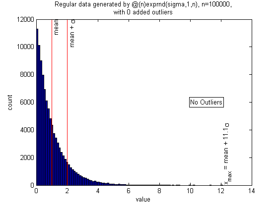
The exponential distribution has a large kurtosis, i.e., it is more likely than the normal distribution to produce points beyond a given number of standard deviations. However, it is in the same Gumbel domain of attraction, so the same outlier detection algorithm can be used. Here the spacing algorithm correctly finds that there are no outliers (the whole sample is from the exponential distribution), even though the largest point is over 10 standard deviations above the mean. (almost always correct; to do: run simulations to determine failure rate)

clf
n = 1e5;
sigma = 1;
randfunc = @(n)exprnd(sigma,1,n);
N = 50; alpha = 0.05; xcenter = 0; mingap = 0;
nout = 0;
pictureoutliers(randfunc,n,nout,xcenter,N,alpha,mingap)

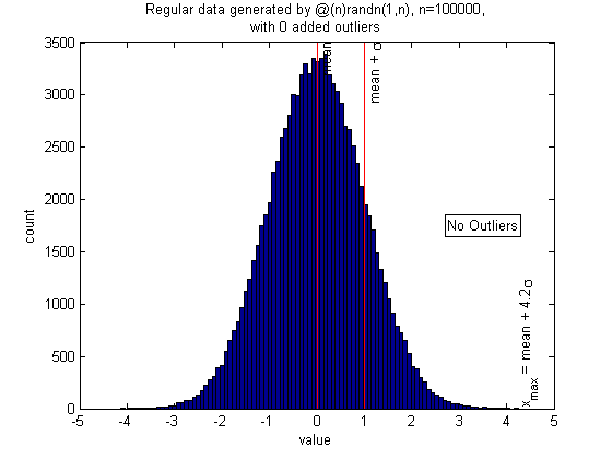
Correctly identifying non-outliers: Normal distribution with no outliers

Same problem, with normal distribution

n = 1e5;
randfunc = @(n)randn(1,n);
N = 50; alpha = 0.05; xcenter = 0; mingap = 0;
nout = 0;
pictureoutliers(randfunc,n,nout,xcenter,N,alpha,mingap)

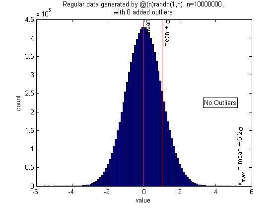
Normal distribution, very large sample size, but no outliers

If your sample size is very large, such as 10⁷, you are likely to get some points greater than 5 standard deviations, even though they are all from the same distribution. But they are correctly identified as non-outliers. I don't have to adjust the threshold by hand; the algorithm finds it itself.

(warning: this requires a lot of memory and may be slow to run)

n = 1e7;
randfunc = @(n)randn(1,n);
N = 50; alpha = 0.05; xcenter = 0; mingap = 0;
nout = 0;
pictureoutliers(randfunc,n,nout,xcenter,N,alpha,mingap)

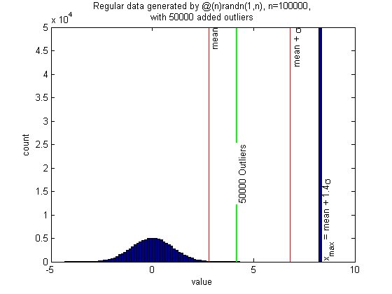
Normal distribution with large numbers of outliers

Now, let's add arbitrary numbers of outliers. Here there are n = 10⁵ normally distributed regular points, and n/2 outliers, which are 2 times the maximum of the regular sample. The sample standard deviation is highly inflated by the large number of outliers. The algorithm correctly places the threshold just above the regular data, and correctly counts the number of outliers.

n = 1e5;
randfunc = @(n)randn(1,n);
N = 50; alpha = 0.05; xcenter = 0; mingap = 0;
nout = n/2;
pictureoutliers(randfunc,n,nout,xcenter,N,alpha,mingap)

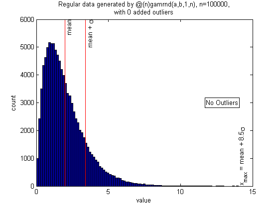
Gamma distribution with no outliers

Another example of a skewed distribution with large kurtosis.

n = 1e5;
a = 2; b = 1; % shape and scale parameters for gamma distribution
randfunc = @(n)gamrnd(a,b,1,n);
N = 50; alpha = 0.05; xcenter = a*b; mingap = 0;
nout = 0;
pictureoutliers(randfunc,n,nout,xcenter,N,alpha,mingap)

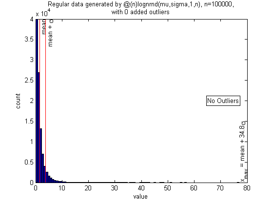
Lognormal distribution with no outliers

This is a skewed distribution with very high kurtosis, but again the algorithm (almost always) correctly finds that there are no outliers, even though the largest regular point is 30 or 40 standard deviations above the sample mean.

n = 1e5;
sigma = 1; mu = 0;
randfunc = @(n)lognrnd(mu,sigma,1,n);
N = 50; alpha = 0.05; xcenter = 0; mingap = 0;
nout = 0;
pictureoutliers(randfunc,n,nout,xcenter,N,alpha,mingap)

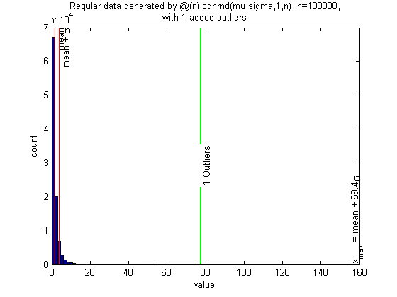
Lognormal distribution with one outlier

However, when a single outlier is added to the lognormal distribution (at 2 times the largest regular point), it is correctly identified. (almost always; to do: run simulation and determine failure rate)

n = 1e5;
sigma = 1; mu = 0;
randfunc = @(n)lognrnd(mu,sigma,1,n);
N = 50; alpha = 0.05; xcenter = 0; mingap = 0;
nout = 1;
pictureoutliers(randfunc,n,nout,xcenter,N,alpha,mingap)

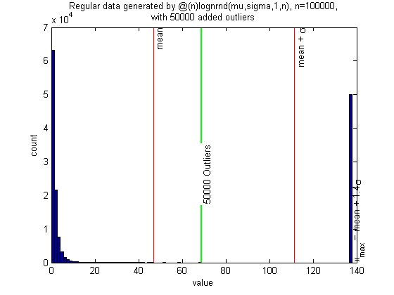
Lognormal distribution with a lot of outliers

The algorithm also works on the lognormal distribution with a large number of outliers.

n = 1e5;
sigma = 1; mu = 0;
randfunc = @(n)lognrnd(mu,sigma,1,n);
N = 50; alpha = 0.05; xcenter = 0; mingap = 0;
nout = n/2;
pictureoutliers(randfunc,n,nout,xcenter,N,alpha,mingap)

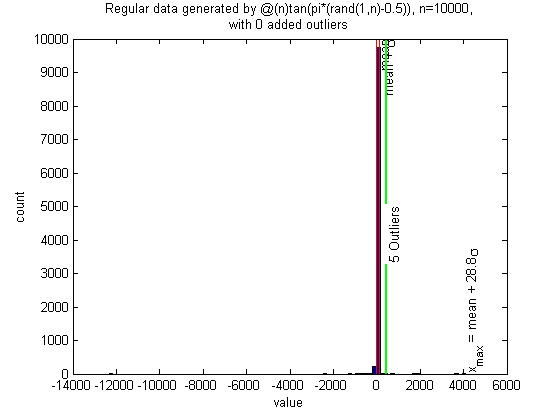
But this is a distribution where it may fail

This is a Cauchy distribution, which is heavy-tailed, violating the necessary assumption. All the data are generated from the same distribution, but outliers may be falsely identified.

n = 1e4;
randfunc = @(n)tan(pi*(rand(1,n) - 0.5));
N = 50; alpha = 0.05; xcenter = 0; mingap = 0;
nout = 0;
pictureoutliers(randfunc,n,nout,xcenter,N,alpha,mingap)

To be continued

Under construction: extreme-value theory and justification of the spacing algorithm.

Author:
Katherine T. Schwarz
Department of Physics, University of California, Berkeley
December 2008

Published with MATLAB® 7.6